Structural images are smoothed by applying a filter, in this case a 3D Gaussian kernel ^[3], to the image. Smoothing increases the signal-to-noise ratio of data by filtering the highest frequencies from the domain: i.e. removing the smallest scale changes among voxels. Hence making the large scale changes more apparent, especially as there is some inherent variability in location and reduce spatial differences between subjects. The trade-off being losing resolution by soothing.

Acts as a preliminary step as it increases speed and accuracy of diagnosis. It removes the non-cerebral tissues like skull, scalp, and dura from brain images. A simple skull stripping algorithm (S3)^[1] based on brain anatomy and image intensity characteristics is shown below:

1. Median Filtering: A \(3 \times 3\) window is passed over the input image, averaging the pixels in that window to be the pixel contrast.
2. Threshold \(T\) estimation: The boundary rectangle of the brain skull is produced from the principle that the skull has an intensity greater than the initial mean intensity value \(T_i\). The final mean value, \(T_f\) is calculated from averaging the pixels within that boundary. The region of brain membrain is selected based on the assumption that the membrane is less that \(T_f\). Then the average of \(T_i\) and \(T_f\) gives us \(T\).
3. Binarization using T: All gray values of the skull are greater than \(T\) are set to a binary 1 and those less than are set to a binary 0.
4. Opening Morphology: The pixels are eroded \(1 \rightarrow 0\) in a \(13 \times 13\) filter to separate the skull from the brain.
5. Finding largest connected component: As the largest connected component is necessarily the brain, the largest area pixel count is isolated.
6. Closing morphology: A \(21 \times 21\) filter fills in any gaps along the edge of the cranium.
7. Mask previous: Using the binary filter anything classed as 0 is removed from the image.

• Each slice is clipped first by restricting the top 1% from the top and bottom of the pixel densities.
• Then for each pixel in the slice the mean of the image is subtracted from the intensity value and divided by the standard deviation

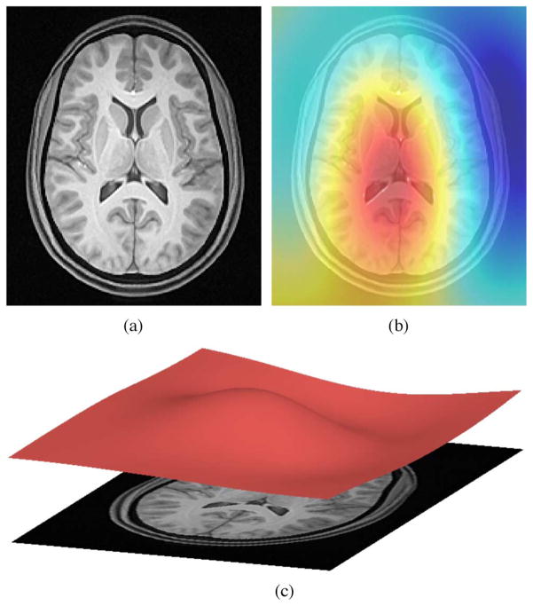
One of the challenges in working with MRI data is dealing with the artifacts produced either by inhomogeneity in the magnetic field or small movements made during scan time. This results in an intensity gradient over the image that can easily lead to misclassification. The stronger the magnetic field strength, the higher the bias field. Beyond 1.5T magnetic field strength can considerably affect MRI analysis.

n4ITK bias correction on all T1 and T1C images in the dataset removes the intensity gradient on each scan, as it estimates the bias field uisng several algorithms and then reapplies that field in reverse to alter the image back to a steady state.