What are SVMs?

Support Vector Machine (SVM) refers to a supervised machine learning algorithm which can be used for both classification or regression challenges.[1]
SVM performs classification by finding the hyperplane that maximises the margin between two classes. In the problem of classifying MRI brain tumour images the two classes can be, for instance, malignant and benign tumour images. Support vectors define the hyper-plane.[15]

Example of a very simple SVM[13]

What are the goals of SVM?

    The goal of support vector machines is to find the hyper-plane (or function) that:
  • separates the two classes (benign tumours and malignant tumours)[1]
  • maximises the distances between nearest data points (from either class) and itself[1]
  • correctly classified unseen examples[2]
This hyper-plane is named the optimal separating hyperplane.[2]

How do they work on linearly separable classes?

If the classes are linearly separable then there must exist a linear hyper-plane that divides the classes accurately. The task therefore its to find this linear optimal separating hyper-plane.
The linear hyper-plane can have the primal form: $$ f(x) = w^Tx + b $$ There is also the dual form: $$ f(x) = \sum_{i}^{N}\alpha_{i}y_{i}(x_{i}^Tx) + b $$

    Where:
  • \(b\) is the bias
  • \(w\) is a (primal) weight vector
  • \(\alpha\) is a (dual) weight vector
  • \(y_{i} \in \{-1, +1\}\)
  • \(x_{i}\) is a support vector
[17]

Example of an SVM trained to classify linearly-separable classes.[11]

How do they work on non-linearly separable classes?

When the classes are non-linearly separable it makes more sense to use the dual form of classifier. However, a kernel is also needed. A kernel is a mathematical function that transforms a low-dimensional input space into a high-dimensional space, allowing the modified classes to become linearly separable[1].
For a kernel \(K(x_{i}, x)\), the dual classifier becomes[17]: $$ f(x) = \sum_{i}^{N}\alpha_{i}y_{i}K(x_{i}, x) + b $$

Example of an SVM with non-linearly-separable classes.[12]

What are common kernels?

Some examples of kernels are shown below:

Linear [2]

$$K(x_{i}, x) = x_{i}^Tx$$

Quadratic [2]

$$K(x_{i},x) = (1 + x_{i}^Tx)^2$$

Polynomial [2]

$$K(x_{i},x) = (1 + x_{i}^Tx)^d$$

Radial Basis Function[14]

$$K(x_{i},x) = exp(-\gamma||x_{i}-x||^2)$$

Note that there are variations of these.

What features do we extract from MRI images?

Once images have been pre-processed the next step is to extract numerical features. The choice of numerical features are important as they will determine the success of any machine learning model.

    Features can be grouped into:
  • Grey-scale features: these include mean, variance, standard deviation, skewness and kurtosis
  • Texture-features: these include entropy, dissimilarity, inverse, energy, contrast and IDM
  • Symmetric feature: the exterior symmetry
Once features are obtained PCA (Principle Component Analysis) can reduce the number of features needed. This is useful because excessive features increase memory use and computation time.[4]

How can we extract these features?

Below are two particular approaches to feature extraction found in the referenced research papers.

GLCM

GLCM is a widely used texture feature extraction technique.[6] GLCM stands for Grey-Level Occurence Matrix and it is a statistical method of examining texture that considers the spatial relationship of pixels. The GLCM function generates a matrix by finding pairs of pixels with specific values and in specified spatial relationships. Statistical values are then calculated using the matrix.[5]
Generated features include contrast, homogeneity, correlation, energy, and difference entropy.[6]

Wavelet Transform & SGLDM

By using 2D wavelet transformation an MRI brain image is decomposed into four sub-bands. The sub-band which has the histogram with maximum variance is selected for further processing. This means that you capture the clearest appearance of changes between different textures.
The selected sub-band is processed by the spatial Grey-Level Dependence Matrix (SGLDM) proposed by R.M.Haralick.
    By applying the SGLDM, 13 features are computed[7]:
  • entropy
  • contrast
  • information measure of correlation I
  • correlation
  • inverse difference moment
  • sum variance
  • variance
  • angular second moment
  • sum entropy
  • difference variance
  • difference entropy
  • sum average
  • information measure of correlation IT

How do we use extracted features to train an SVM?

After features have been extracted for each MRI image in the training data, data points need to be constructed (where a data point corresponds to an image). Each data point will contain all the values for each feature and the classification of the image (malignant or benign) as a -1 and +1.[3]
The SVM is then trained using each data point. For the dual classifier training involves learning the values in \(\alpha\) to determine the hyper-plane (and which data points are its support vectors).
One modern algorithm used for training a dual classifier is Co-ordinate Descent. For each \(i \in \{1 .. n\}\), iteratively, the co-efficient \(\alpha_{i}\) is adjusted in the direction that reduces the error. Then, \(\alpha\) is projected onto the nearest vector of co-efficients that satisfies the given constraints (typically Euclidean distances). This is repeated until near optimal coefficients are obtained. [16]

How do we test and measure performance of an SVM?

Given a trained SVM testing involves 'plotting' unseen data points (MRI images) in the space, and seeing if the SVM's classification of the data point matches the correct classification.

    The options when classifying any data point, for the problem of classifying brain tumours as benign and malignant, are as follows[4]:
  • True positive (TP): Malignant brain tumour correctly identified as malignant
  • False positive (FP): Benign brain tumour image incorrectly identified as malignant
  • True negative (TN): Benign brain tumour image correctly identified as benign
  • False negative (FN): Malignant brain tumour incorrectly identified as benign
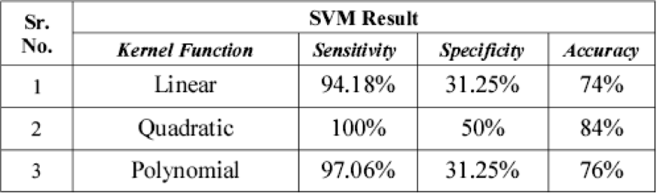
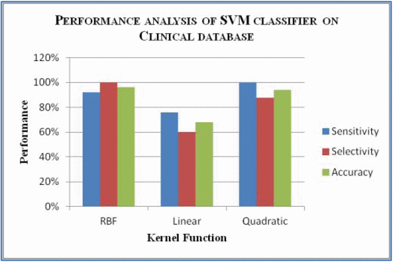
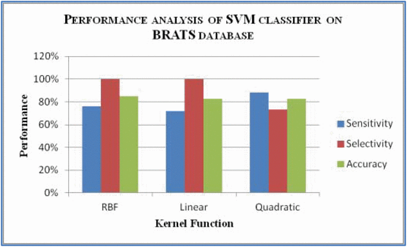
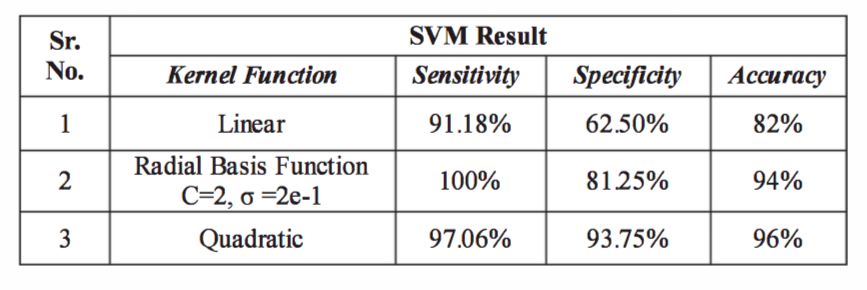
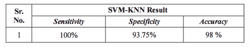
    The following statistical measures can be taken:
  • Sensitivity: TP/(TP + FN) * 100%
  • Specificity: TN/(TN + FP) * 100%
  • Accuracy: (TP + TN)/(TP + TN + FP + FN) * 100%
Sensitivity can be thought of as the proportion of malignant brain tumours correctly identified, and specificity as the proportion of benign brain tumours correctly identified. One can argue that sensitivity is more important than specificity since it is time critical to identify malignant tumours.

How do SVMs perform at classifying MRI brain images from MRI images?

    Across papers referenced, SVMs have been used in classifiying:
  • Normal vs Abnormal MRI brain images
  • Benign vs Malignant MRI brain tumour images
  • Low grade glioma vs High grade glioma MRI brain tumour images
All of which involve similar feature extraction and training/testing procedures. The results of training SVMs for these purposes are shown below. Given that the SVMs appear to achieve a high accuracy in classifying malignant and benign brain tumours from MRI images, SVMs may be incredibly useful for assisting doctos with time-critical diagnosis.

Other considerations

This page deals with a generalised approach to using SVMs for MRI brain image analysis, however, there are other specific considerations:

Overfitting

When training an SVM it is important that the model does not overfit to the training data. When an SVM overfits the error on the training set becomes very small, but becomes large when presented with unseen instances.
One method of avoiding overfitting is K-fold cross validation. The idea is to create a K-fold partition of the whole dataset, repeat K times to use K−1 folds for training and a left fold for validation, and finally average the error rates of K experiments.7

Choice of kernel values

When choosing the RBF as the kernel there is the choice of \(\gamma\) to be made. The \(\gamma\) parameter determines how much a single training example influences the SVM. A lower value means that the influence is greater. 9
Similarly, when choosing a polynomial kernel there is the choice of \(d\). Choosing \(d = 2\) is quite common (and is a quadratic kernel), but choosing a high value of \(d\) will cause \(K(x_{i}, x)\) to tend to a value of 0 or infinity, thus, not proving as effective.[10]

Hybrids

One of the results shown above is from a SVM-KNN hybrid[8]. The performance of this hybrid shows that SVM may be best used with other methods to optimise the accuracy of an MRI brain tumour classifier.

Footnotes