What is a Neural Network

A neural network is a system made up of a number of simple, highly interconnected processing elements which process information by their dynamic state response to external inputs.[1]

Neural nets are usually made up of a series of layers, each of which contains a selection of 'nodes' which create an 'activation function'.

    There are typically 3 'types' of layers:
  • Input
  • Hidden Layers
  • Output
Data (patterns) enter the network via the input layer, are passed through one or more hidden layers and the result is given in the output layer. Neural nets enable computers to learn to perform a task by analysing training samples. Often, this is done using data which has been labelled so corrections in the model can be made. This is called supervised learning.

A structural diagram showing layers of a neural network.[13]

What is a PNN?

A Probabilistic Neural Network (PNN) is a type of feedforward neural network and also a Radial Basis function network, which has the majority of uses in pattern recognition and image classification [2]. PNNs usually consist of four layers; an input layer, hidden layer/ radial basis layer, summation layer, and output layer with each feeding it's output to the next. From the papers referenced, they all use slightly different implementations of the layers, for example, some have multiple nodes in the output layer but others only have one.

The abstracted layer structure of a PNN [7]

What are the Advantages of PNNs?

    PNNs have a number of advantages that make them more favourable to use when classifying tumours [6]:
  • They are very quick to train.
  • They have a permanent parallel structure.
  • They are guaranteed to classify an image and this classification will be optimal as the data set grows.
  • Training samples can easily be added or removed without considerable retraining.

How are PNNs Implemented?

As is formerly mentioned, PNNs contain an input layer and an output layer. In this sense they are similar to other neural networks as the number of input nodes corresponds to the number of pixels recieved; the activation of an input node depends on the brightness of the pixel for that node. The number of output nodes is determined by the number of classes the network has to determine between.

Hidden Layer/Radial Basis Layer

PNNs work by using the Radial Basis layer to calculate distance from the input vectors to the training vectors. This is done using a Radial Basis Function (RBF)[1]. The RBF has several different implementations in the papers referenced, one of which is shown below [5]:
The output vector of the Radial Basis layer, \(a\), is given as: $$a_i = radbas(||W_i − p|| .∗ b_i)$$ Where \(W\) is the weight vector, \(p\) is the input vector (so \(||W_i − p||\) is the distance vector between the input and weight.) and \(b\) is a bias vector. This paper represents the distance criterion with respect to a center as:
$$ radbas(n) = e^{-n^2} $$

Summation Layer

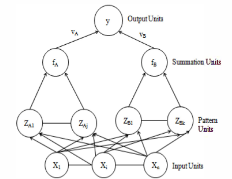
The network then passes data from the RB layer to the summation layer which calculates the closest distance between the training images, and the input image and classifies the image based on the closeness of the data. This is usually done using Bayesian Theory [4]. Some of the sources show the summation layer performing the following calculations [7] [8] [9]

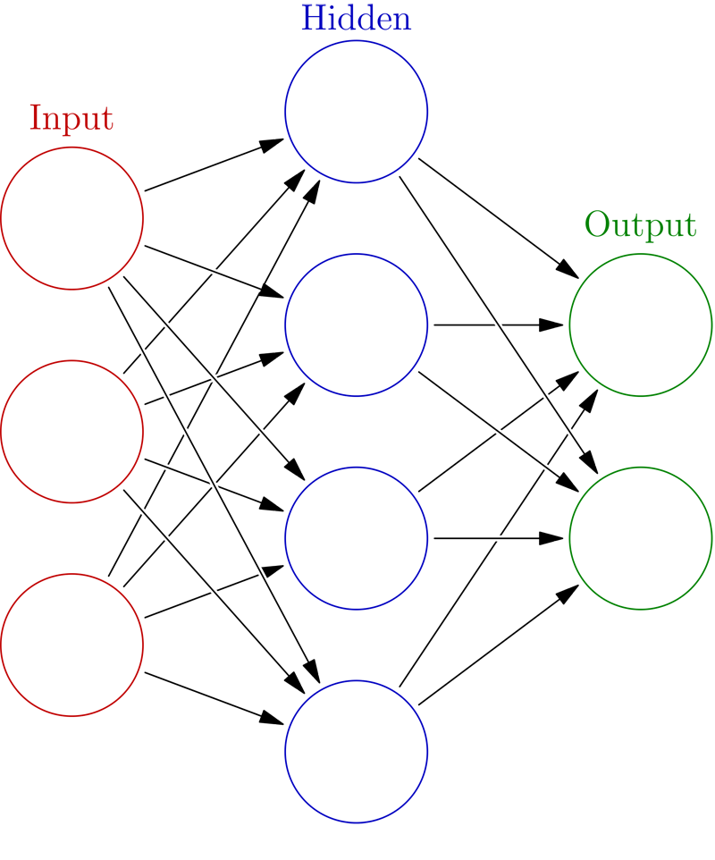
The PNN separates the input vectors into classes. An input vector is classified into a class \(A\) by the equation:

$$ P_A C_A F(x)_A > P_B C_B F(x)_B $$ Where
\(P_A\) - Priori probability of occurrence of patterns in class
\(C_A\) - Cost associated with classifying vectors
\(F(x)_A\) - Probability density function of class A given by the equation $$ F(x)_A = \frac{1}{(2π)^{\frac{n}{2}} \ \sigma^n \ m_n} $$ with $$\sum_{i = 1}^m exp[-2 \ \frac{(x - x_A)^r (x - x_{Ai})}{\sigma^2}]$$ Where
\(x_{Ai}\) - ith training pattern from class A
\(n\) - Dimension of the input vectors
\(\sigma\) - Smoothing parameter (corresponds to standard deviation of gaussian distribution)


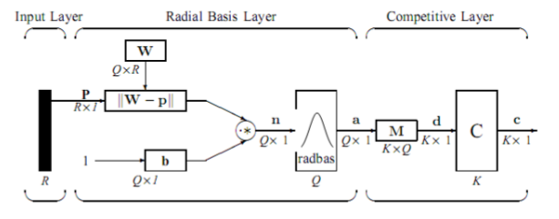
The Mathematical representation of a PNN as a structural diagram.[5]

What Role do PNNs Play in Medical Imaging?

In the medical context, the PNN carries out the MRI classification in the automated procedure of detecting and analysing brain tumours. They can determine between many types of tumour, for example, benign, metastatic, and malignant as well as normal, non-tumor containing images. Their implementation determines the different classes of tumour they can distinguish between as does the training data supplied. The PNN is used in the last stage of the classification steps which is usually done before segmentation.

A diagram to show the stages that occur in the classification process of a brain tumour[7]

Testing PNNs with BRATS benchmark

A paper about PNNs and classification[8] provides some results of a tested PNN implementation on a BRATS dataset. We also gained some classification data from the BRATS dataset[11]. The images in the table below are just slices of the data, of which there were 127 for each brain. More information can be found about the slices on the overview page.

Our Classification Results

Input Image Segmented Image Type of Tumour Tumour Affected Area (mm3)
High Grade Glioma
  • Necrosis: 15476
  • Edema: 35716
  • Non-Enhancing Tumor: 12689
  • Enhancing Tumor: 50134
Low Grade Glioma
  • Necrosis: 105
  • Edema: 48317
  • Non-Enhancing Tumor: 37090
  • Enhancing Tumor: 8726

This tells us that we may be on the way to writing computer programs that could do what a radiologist does, and eventually write software that saves doctors a great deal of time and many lives.

Footnotes